A Quick Introduction to R

By Matteo Dell'Omodarme and Giada Valle

The aim of this article is to introduce the R environment and to show its basic usage. Only a small share of the huge amount of software features can be described here. We chose to put special emphasis on the graphical features of the software, which can be appealing particularly to novel users.

Overview of R

R (http://www.r-project.org) is an integrated suite of software tools for data manipulation, calculation, and graphical display. It provides a huge set of statistical and graphical techniques such as linear and nonlinear modelling, statistical tests, time series analysis, non-parametric statistics, generalized linear models, classification, clustering, bootstrap, and many others. R is being developed for the Unix, Windows, and MacOS operating systems.

The core of R is an interpreted computer language that allows branching and looping as well as modular programming using functions. Most of the user-visible functions in R are written in R, but it is possible to interface to procedures written in C, C++, or FORTRAN for efficiency. Elementary commands consist of either expressions or assignments. If an expression is given as a command, it is evaluated, printed, and the value is lost. An assignment also evaluates an expression and passes the value to a variable, but the result is not automatically printed. Commands are separated by either a semicolon or a newline.

The R language was developed from the S language - which forms the basis of the S-Plus systems - and it is very similar in appearance to it. Most of the code written in S can run in R with no or little modification. While S-Plus is proprietary software, R is free software distributed under a GNU-style copyleft, and an official part of the GNU project. All these features have made it very popular among academics.

Features, Extensibility and Documentation

The main features of R include:

• data handling and storage facility
• operators for calculations on arrays and matrices
• a large set of tools for data analysis
• graphical facilities for data analysis and display
• a well-developed, simple, and effective programming language

These features are extended by a large collection of user-supplied packages. There are more than twenty packages supplied by default with R ("standard" and "recommended" packages) and many others (about 1000) are available through the CRAN (Comprehensive R Archive Network) family of Internet sites and elsewhere.

An enormous amount of background information, documentation, and other resources is available for R. CRAN is the center for information about the R environment. The documentation includes an excellent internal help system, some user guides (in particular An Introduction to R), a FAQ list , and a number of textbooks (see the R project Web page for a comprehensive bibliography.) In addition to the textbooks, the R project Web page also hosts several contributed tutorials and manuals.

As final remarks, we want to point out two software features not mentioned above. First, R can also be run non-interactively, with input from a file and output sent to another file. Second, there are several packages available on CRAN to help R communicate with many database management systems. They provide different levels of abstraction, but all have functions to select data within the database via SQL queries, and to retrieve the result as a whole or in pieces.

Installing R

The latest copy of R, as well as most contributed packages, can be downloaded from the CRAN Web site. Binaries for several platforms and distributions are available at http://cran.r-project.org/bin/ . Source code can be downloaded at http://cran.r-project.org/sources.html . Note that one needs a FORTRAN compiler and a C compiler to build R. (Perl version 5 is needed to build the R documentation.)

Installation from source is straightforward. Download the source code (the latest is R-2.4.1.tar.gz), extract it, and change directory to the one extracted from the archive:

$ tar zxf R-2.4.1.tar.gz
$ cd R-2.4.1 

Then, issue the usual commands:

$ ./configure
$ make
$ make install  

This will perform the compilation and the installation of binaries and libraries (typically in /usr/local/bin/ and /usr/local/lib/R/).

The tarball contains all the standard and recommended packages. Once this base version is installed, other user-contributed packages can be downloaded from http://cran.r-project.org/src/contrib/PACKAGES.html. CRAN Task Views allow browsing packages by topics for a systematic installation. A downloaded contributed package can be installed with the following command (which needs superuser privileges):

$ R CMD INSTALL
package-name.tar.gz

Running R and Its Help System

To start a R session, simply type the following at the shell prompt:

$ R

This command invokes the R environment, displays a standard disclaimer, shows some information about the main usage of the software, and prompts for user input:

R version 2.4.1 (2006-12-18)
Copyright (C) 2006 The R Foundation for Statistical Computing
ISBN 3-900051-07-0
  
R is free software and comes with ABSOLUTELY NO WARRANTY.
You are welcome to redistribute it under certain conditions.
Type 'license()' or 'licence()' for distribution details.
 
  Natural language support but running in an English locale
 
R is a collaborative project with many contributors.
Type 'contributors()' for more information and
'citation()' on how to cite R or R packages in publications.
 
Type 'demo()' for some demos, 'help()' for on-line help, or
'help.start()' for an HTML browser interface to help.
Type 'q()' to quit R.
 
> 

Like other powerful analysis tools, such as ROOT (GNU Lesser General Public License) and IDL (proprietary software), the interaction with the software is via command line. This approach, which can be intimidating for the novice user, reveals all its power once one has mastered a few basic syntactic rules.

A good example of this is the analysis of the excellent internal help system. It can be browsed in HTML format by running the command:

> help.start()

which opens the default browser at the following page:

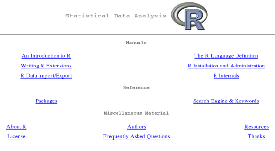
Starting from the top, there is the Manuals zone, from which one can access six documentation papers included in the standard distribution. The most useful for a beginner is An Introduction to R, which introduces the language, its syntax, and its usage in several analyses. A careful reading of this document is strongly advised for every person seriously interested in this software environment. The other papers are more technical, and are intended for advanced users.

From the Reference section, the user can browse the list of installed packages, looking for a specific function in a specific package (from a link on the left), or search the manual pages by keyword (from a link on the right). The search engine is written in Java, and invoked by Javascript code, so they will need to be enabled in the browser.

A Simple Introductory Session with R

A systematic introduction to the syntax of R is far beyond the aim of this article. However, in this section, we'll explore some basic commands and features of the language.

As mentioned previously, either an expression or assignment can be entered. Here is an example:

> 3 + 2
[1] 5
 
> x <- 3 + 2
> x
[1] 5

In the first line, a simple arithmetic expression is entered; the software evaluates it and returns the result. The second example shows an assignment; the result of the previous calculation is now assigned to the variable x. In this last case, two things should be noted: first, the software does not return anything, and the user can inspect the value of the variable by entering its name. Second, the assignment operator is "<-", which consists of the two characters '<' (less than) and '-' (minus) occurring strictly side-by-side, which points to the object receiving the value of the expression.

The language allows construction and manipulation of vectors and matrices. To set up a vector named y, consisting of the two numbers 1 and 3, use the R command:

> y <- c(1, 3)

where we used the concatenation function c(). When vectors are used in arithmetic expressions, the operations are performed element by element. In the case of vectors occurring in an expression that are not of the same length, the value of the expression is a vector with the same length as the longest vector. Shorter vectors in the expression are recycled, until they match the length of the longest vector. (A constant is simply repeated.) In the following example, we square the elements of y and add one to both of them:

> y^2 + 1
[1]  2 10

The user can select vector elements by appending to the name of the vector an index vector in square brackets:

> x <- c(1, 3, 5, 8, 2)
 
> x[3]
[1] 5
  
> x[c(1, 3)]
[1] 1 5

In the first example, only the third element is selected, while, in the second, we extract the first and third elements.

The index vector can also be a logical vector. In this case, it must be of the same length as the vector from which elements are to be selected. The values corresponding to the logical value TRUE in the index vector are selected, and those corresponding to FALSE are omitted. In the following two examples, we use logical vectors to extract the elements of x greater than 4 and the elements greater than 2 and lesser than 10:

> x > 4
[1] FALSE FALSE  TRUE  TRUE FALSE
 
> x[x > 4]
[1] 5 8
 
> x[x > 2 & x < 10]
[1] 3 5 8

In this second example, we used the logical operator "&" (AND). As a final remark, a minus sign can be used to select all the components except the ones in the index vector:

> x[-c(1, 4)]
[1] 3 5 2

Matrices are built using the function matrix():

> A <- matrix( c(1, 3, 5, 6, 8, 11), nrow=3 )
  
> A
     [,1] [,2]
[1,]    1    6
[2,]    3    8
[3,]    5   11

where nrow=3 is the desired number of rows. Note that the matrix is filled by column.

Individual elements of a matrix may be referenced by giving the name of the matrix followed by index vectors in square brackets, separated by commas. If any index position is empty, then the full range of that dimension is taken. In the following example, we select: the element of A in the second row, first column; all the third row; all the second column:

> A[2, 1]
[1] 3
 
> A[3, ]
[1]  5 11
 
> A[ , 2]
[1]  6  8 11

R Graphical Features

Many users will come to R mainly for its graphical facilities, which are an important and extremely versatile component of the environment. It is possible to use the facilities to display a wide variety of statistical graphs, and also to build entirely new types of graph.

Some of the examples below are performed on random generated data; in each of them, the seed of the random generator is set for reproducibility (with the function set.seed()). We'll start by considering a simple bidimensional scatterplot. The values in x come from the numerical sequence 1, 2, ..., 40, which is obtained using the ":" operator, while y contains 40 Gaussian random numbers (by default by a sampling distribution with mean 0 and standard deviation 1):

> set.seed(100)
> x <- 1:40
> y <- rnorm(40)

The plot is then obtained by calling the function plot(). Several options can be entered, changing the type of the graph (point, line, both), the color of the lines or the symbols, the weight of the lines, the axes' label, etc. In the example below, we plot a default point-style graph as well as line-type version of the plot (not shown):

> plot(x, y)
> plot(x, y, type="l")

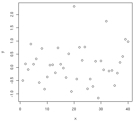
"Hard" copies of the graph can be generated in several formats. PNG, PostScript, and PDF outputs are obtained by calling respectively the functions png(), postscript(), and pdf(), before the graphics call. Besides several optional control parameters, in all these functions the user must enter the name of the output file. The above figure is obtained with the following commands:

> png("graph1.png")
> plot(x, y)
> dev.off()

The function dev.off(), which should be called at the end of all the graphics calls, closes the active graphical device (the one opened with png()), and saves the file graph1.png.

In the next example, let us imagine that y's datapoints are extracted from different groups. In this case, a common graphic visualization is a boxplot. Let us also suppose that the data come from four different groups, each one containing 10 objects. We'll introduce a group factor (using the function gl()), which assumes a value of 1 for the first 10 objects, value 2 for the next 10, and so on. The boxplot is displayed in the following figure:

> group <- gl(4, 10)
> boxplot(y ~ group, xlab="Group")

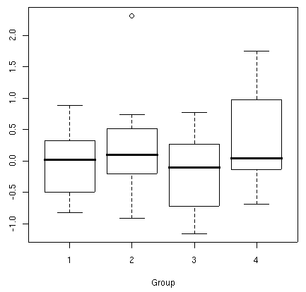
The function boxplot() is used with two arguments: a formula describing the structure of the data (response data on the left side, grouping factor on the right, separated by a tilde), and a graphical option that sets the x-axis label.

An alternative use of the dataset is the visualization via scatterplot, with the four groups identified by different symbols:

 
> plot(x, y, pch=as.numeric(group))
> legend("topleft", c("g1", "g2", "g3", "g4"), pch=1:4)

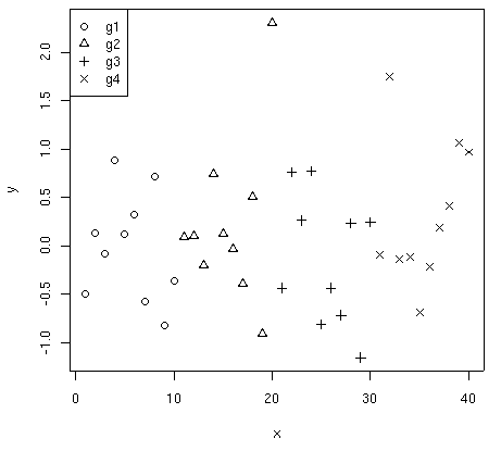
The option pch allows the selection of several symbols. Here, the object group number (obtained by calling the as.numeric() function on the group factor) is used to select the symbol among the first four, assigning symbol 1 (circle) to the first ten objects, symbol 2 (triangle point-up) to the next 10, etc. The example also shows how to insert a legend in a plot. The three arguments of the legend() function are: the location, the labels, and a distinctive mark for each label (in this case, the symbols of the four groups).

The points() function can be used to add a symbol to an active graphical device (resulting plot not shown):

> points(12, 1.5, pch=19, col="red")
> text(12, 1.5, "Demo point", col="red", pos=4)

This arguments of the function are the coordinates of the points to plot, the type of the chosen symbol (pch=19 identifies a filled circle), and the color code. The text() function is used to add a label in a plot. Most of its arguments are similar to those of the points() function, since text() takes the coordinates of the label, the label to be inserted, the color code, and the text position specifier. (pos=4 indicates a position right of the specified coordinates.)

In the third example, we show a barplot. Let us consider two series of frequencies a and b, each one with three elements. The graphic is constructed by calling the barplot() function:

> a <- c(10, 13, 7)
> b <- c(4, 9, 10)
> barplot(rbind(a, b), beside=TRUE, names=c("A","B","C"), col=c("red","green"))
> legend("topright", c("first", "second"), fill=c("red", "green"))

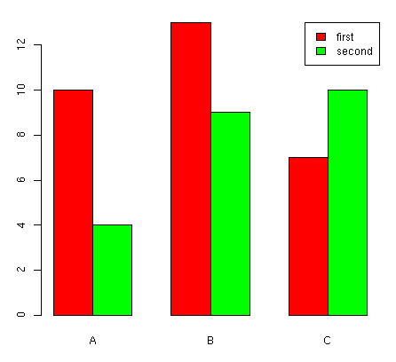
The rbind() function is used to combine the two series of frequencies by row, in order to plot them together. The option beside is used to show the bars juxtaposed (not stacked), while the option name is used to specify the labels to be plotted below each group of bars. The last option of legend() requests, in this case, a filled box with the same color of the bar corresponding to the label.

In the following two examples, we show some graphical facilities for 3D data. To plot the values in variable z on a 36 x 36 x-y grid (x = 1, 2, ..., 36, y = 1, 2, ..., 36), a filled contour plot can be helpful (the example data are randomly generated):

> set.seed(100)
> z <- matrix(rnorm(36*36), nrow=36)
> x <- 1:36
> y <- 1:36
 
> filled.contour(x, y, z)

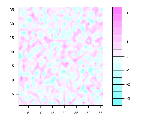
The filled.contour() function requires the z values, entered in matrix form.

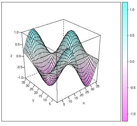
In the last example, we showed a classical 3D plot; in this case, we'll use a function defined in the add-on 'lattice' package, which is installed but not loaded by default. The library() function is therefore used to load the required package. In the example, we'll plot the following mathematical function:

z = sin(x/18 pi) * cos(y/18 pi)      

As in the previous example, we need to define the values of z on a regular grid. Let us use the same grid as before (x = 1, 2, ..., 36, y = 1, 2, ..., 36). The matrix of z values is easily obtained by outer product (operator "%o%"):

> z <- sin(pi*(1:36)/18) %o% cos(pi*(1:36)/18)

The wireframe() function is then called. The drape option drapes the wireframe in color, while the scale option is used to insert the tick marks.

> library(lattice)
> wireframe(z, drape=TRUE, xlab="x", ylab="y", scale=list(arrows=FALSE))

Many other plotting functions are available. For the univariate case, we have histograms and density plots; for multivariate cases, there is a huge number of advanced plots, related to the available analysis techniques, such as stars plots, autocorrelation plots, ternary plots, scatterplot matrices, mosaic plots, dendrograms, principal component projections, discriminant analysis plots, correspondence analysis plots, survival estimated curves, etc. They rely on more advanced statistics methods, which cannot be introduced here. Interested readers can refer to the available documentation, listed in the last section of this article.

Conclusions and Further Readings

The R environment, briefly presented here, is an extremely powerful tool for statistical analysis and data manipulation, released under GNU General Public License. Thanks to the myriad of contributed packages, there is virtually no analysis that cannot be tackled using existing functions. Even in the rare case in which no software is available to deal with an unusual problem, users can implement the needed routine on their own (either in R, or by interfacing C or FORTRAN code).

Although many features of the programs can be better appreciated by more advanced users (mainly statisticians), even novice users can benefit from a basic usage of the environment. In this overview, we chose to dedicate special attention to the introduction of its (basic) graphical facilities, in the hope of providing a gentle approach to an environment that is frequently, but perhaps unfairly, considered as intimidating.

Other statistical packages are available on the market (e.g. SPSS, Stata, SAS, Statistica, S-plus and MINITAB), but their single-user licences cost more than US $1,000. By comparison, R, which combines great power with a free license, is as an invaluable resource for researchers or students involved in data analysis. For the same reason, R can be used with success in statistics courses, either at introductory or at advanced levels. (See, for instance, http://arxiv.org/abs/physics/0601083, where we discuss these topics in detail.)

Readers seriously interested in the software can start by reading An Introduction to R, which systematically presents the language and its syntax, and then check out the contributed documentation on the CRAN website. Some of the available documents are topic-specific, but others are more general. The Web site also hosts many documents in languages other than English.

Several books and papers on R have been printed in recent years. Among them, we would like to point out the first presentation of the environment and a textbook that can be used as an all-purpose reference:

• R. Ihaka and R. Gentleman (1996). R: A language for data analysis and graphics. Journal of Computational and Graphical Statistics 5(3), 299-314.
• W.N. Venables and B.D. Ripley (2002). Modern Applied Statistics with S. Springer-Verlag, New York (4th ed.).

Talkback: Discuss this article with The Answer Gang

Matteo Dell'Omodarme

---

I am a physicist involved with Linux since 1994, when I acted as system and security manager at the Department of Astronomy, University of Pisa (Italy). My current research interests are mainly in Applied Statistics, but I also work as system manager, net manager, web developer and programmer (C, C++, FORTRAN, Php, Tcl/Tk).

Giada Valle

---

I am an astrophysicist mainly interested in galactic evolution; in this subject I develop simulation codes in C/C++ and FORTRAN. I've been using Linux since 1998, when I worked on my degree thesis at the University of Pisa (Italy).